
When Does Deep Learning Make Sense for American Option Pricing?

Evidence from a reproducible American put surrogate-pricing project

Abstract
This article summarizes a completed deep-learning project on American put option pricing, built as a reproducible research workflow and fully documented in the public GitHub repository linked at the end. The question driving it wasn't whether a neural network can fit option prices — of course it can — but whether deep learning adds anything a competent numerical method doesn't already give you. To find out, the project generated a synthetic dataset of 1.45 million American put observations from a validated high-resolution Cox-Ross-Rubinstein (CRR) tree, then pitted several neural architectures against each other and against that tree: a direct multilayer perceptron (MLP), premium-based and constrained residual models, an exercise classifier, a neural Longstaff-Schwartz continuation policy, and an integrated multi-head model.
The headline result is that a financially structured residual network materially improves pricing accuracy, eliminates lower-bound violations, and prices faster in batch than repeated tree valuation — but only inside the domain it was trained on. The broader conclusion is conditional, not triumphant: deep learning earns its place as a surrogate for large, repeated, in-domain valuation workloads. It is not a replacement for numerical pricing, and it doesn't win by default just because it's deep learning.
Introduction
American options are harder to price than European ones for a specific reason: they embed an optimal-stopping decision. At every exercise date, the holder has to weigh immediate exercise against the value of waiting, which turns American pricing into a computational problem before it's ever a machine-learning one. That framing shaped how this project was approached. Rather than reaching for deep learning because the course was about deep learning, the goal was to test whether a financially structured neural network could learn a validated American pricing function accurately enough, honestly enough about its own limits, and with enough of a computational edge to justify using it as a practical surrogate in the right operating environment.
The scope stayed narrow on purpose — American put options only. That kept the experiment identifiable, kept the financial constraints clean, and lined the project up with the existing literature on supervised option pricing and optimal stopping. Real-market datasets don't give you the controlled coverage this kind of experiment needs, so the project used a tested pricing engine to generate synthetic data instead. That trade-off is what made it possible to train against a known target function while keeping exact labels for price, early-exercise premium, continuation value, and the exercise decision itself.
What the project did
The work moved through nine Jupyter notebooks and a supporting source-code package, each building on the last:
1. Theory notebook — set up the financial problem, the early-exercise premium decomposition, and the research questions the rest of the project would try to answer.
2. Pricing-engine notebook — validated Black-Scholes and CRR pricing, studied convergence behavior, and selected the tree resolution used for production.
3. Data notebook — generated and audited the final synthetic dataset: 1,000,000 core observations, 250,000 boundary-focused observations, and four 50,000-row out-of-domain stress sets, for 1.45 million rows in total.
4. Notebook 04 — trained a direct MLP to predict the normalized American put price. This is the naive baseline the rest of the project measures itself against.
5. Notebook 05 — reframed the problem as predicting the residual above a financial floor rather than the price itself, and turned out to produce the strongest static price model in the project.
6. Notebook 06 — tackled the exercise-versus-continuation decision two ways: a dedicated classifier and a shared price-and-exercise model.
7. Notebook 07 — ran classical Longstaff-Schwartz against a neural continuation-policy variant in a separate, path-based experiment.
8. Notebook 08 — built an integrated multi-head model that produced protected price, direct price, continuation value, and an exercise recommendation from one shared representation.
9. Notebook 09 — pulled the evidence together, tested it against the predefined hypotheses, and answered the central business question.
The organizing principle throughout was to keep the numerical method as the reference layer and treat deep learning as a surrogate to be earned, not assumed.
Figure 1 — Static pricing models on the common test set. The constrained floor residual MLP is the strongest static pricing model.

Figure 2 — Exercise-decision models on the common test set. The integrated warm-start exercise head is marginally ahead, but the specialist classifier remains a clean exercise-only choice.

Figure 3 — Path-based pricing experiment. Classical Longstaff-Schwartz outperforms the neural variant in this implementation.

Main results
What makes this evidence more convincing than a lot of "deep learning for finance" demos is that the models weren't just compared on average error. They were checked against aligned test data, and judged on financial validity, exercise quality, out-of-domain deterioration, and runtime together — four separate ways for a model to fail.
On the common test set, the constrained floor residual MLP from Notebook 05 came out on top among the static pricing models, with a mean absolute price error of roughly 0.010. Compare that to about 0.078 for the direct MLP, and about 1.34 for the European Black-Scholes proxy used as a naive American substitute. The gap between those numbers is the real finding here: it isn't that a neural network can approximate American prices — plenty of prior work has shown that — it's that how you frame the target matters far more than how elaborate the architecture is. The constrained model also cleared up something the direct MLP couldn't: lower-bound violations, where a naive price prediction can dip below the option's intrinsic value. Once the model is forced to predict a residual above a financial floor, that problem disappears by construction.
The exercise-decision question told a similar story with a smaller margin. The best F1 score came from the integrated warm-start exercise head, only marginally ahead of the specialist exercise-only classifier. In practice that means the choice comes down to what you actually need: if all you want is the exercise recommendation, the specialist classifier is the cleaner deployment; if you need price and exercise decision from the same model, the integrated version is the sensible compromise.
Not every experiment worked out, and it's worth being upfront about that. The path-based comparison in Notebook 07 produced a negative result — classical Longstaff-Schwartz outperformed the neural continuation-policy variant, which showed both higher held-out pricing error and weaker interval behavior. So no, this project doesn't claim that bolting a neural network onto any given valuation method automatically makes it better. Sometimes the classical method just wins.
Out-of-domain performance is the other place where the models had to earn their keep, and here they mostly didn't. Every eligible static neural model deteriorated materially once pushed outside its training range. That's not a reason to write the models off — it's a reason to use them behind domain checks, with a numerical fallback ready for anything that falls outside the trained range. In practice, that range already covers a broad enough span of moneyness, maturity, volatility, interest rates, and dividend yields to handle ordinary operating conditions. The out-of-domain sets are better read as stress tests than as a preview of routine production use.
Figure 4 — Error deterioration outside the training range. Out-of-domain deterioration is material across eligible static neural models.

Business interpretation
The strongest practical case for the surrogate approach isn't accuracy on its own — it's what accuracy buys you computationally. Once trained, the selected static neural models comfortably outrun repeated high-resolution tree valuation on large batches. On the machine used for testing, both the constrained residual model and the integrated model became reliably faster than the project's high-resolution Numba CRR implementation from around 1,000 valuations per job onward. At one million valuations, the constrained residual model finished the workload in roughly 2.4 seconds against roughly 18 seconds for the project CRR, and the integrated model came in at roughly 2.9 seconds.
That's a real speedup, but it only means something in the right context. For a one-off valuation, or a small portfolio, the numerical method is still the sensible choice — there's no batch to amortize the model's training cost against. The use case where this actually pays off is high-volume and repetitive: scenario grids, intraday risk systems, large brokerage operations, options market making, institutional portfolio revaluation, and potentially high-frequency trading, where shaving off latency has real operational value.
Figure 5 — Selected static neural model versus high-resolution CRR on a per-option basis. The neural surrogate drastically reduces marginal valuation time after training.

Figure 6 — Runtime scaling by valuation method. Neural inference becomes relatively more attractive as batch size grows.

Figure 7 — Speedup versus the project CRR. The neural models become faster in sufficiently large jobs.

The lifecycle break-even analysis makes the same point from a different angle, and it's the part of this project I'd flag as most useful for anyone evaluating an "AI speedup" claim elsewhere. A neural surrogate gets fast quickly at runtime, but it isn't free to build — label generation, training, validation, and deployment all cost time up front. Treating runtime crossover (when does inference beat the tree, per job) and lifecycle break-even (when does the cumulative time saved cover the build cost) as two separate questions is what keeps this analysis honest, and it's a distinction that's easy to skip when someone's trying to sell you on AI.
Figure 8 — Estimated annual workload impact. The operational case becomes meaningful in large and repeated valuation workloads.
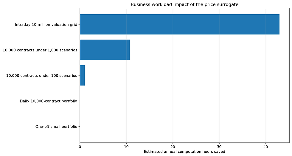
Figure 9 — Lifecycle break-even under different up-front build-cost assumptions.

Conclusion
The conclusion here is conditional rather than ideological, and I think that's the more useful outcome. Deep learning makes sense in this problem when it functions as a financially structured, in-domain acceleration layer for large, repeated American put valuations. It doesn't make sense as a universal replacement for numerical pricing, and it doesn't earn architectural complexity just because complexity is available.
The best-performing model in the whole project wasn't the largest or the most elaborate one — it was the constrained floor residual MLP, which won by combining financial structure with a simpler learning task rather than by throwing more capacity at the problem. The integrated model earned its place when price and exercise information needed to come from a single model. The neural Longstaff-Schwartz variant, on the other hand, didn't earn a deployment case at all — a useful reminder that "neural" isn't automatically "better."
Put simply: deep learning can add real value in option pricing, but only under specific conditions — a validated numerical reference to check it against, a well-defined operating domain, a workload large and repetitive enough to justify the build cost, and financial constraints built into the model rather than bolted on afterward. That's a narrower claim than either the AI-optimist or AI-skeptic version of this story, and I think it's the more accurate one.
Evidence base
All empirical claims in this article are drawn from the public project repository and its final evaluation workflow: github.com/Kamend1/deep_learning_american_option_pricing
References
Black, F., & Scholes, M. (1973). The pricing of options and corporate liabilities. Journal of Political Economy, 81(3), 637–654.
Cox, J. C., Ross, S. A., & Rubinstein, M. (1979). Option pricing: A simplified approach. Journal of Financial Economics, 7(3), 229–263.
Ding, L., Lu, E., & Cheung, K. (2025). Deep learning option pricing with market implied volatility surfaces.
Elbayed, Z., & Qadi El Idrissi, A. (2025). Deep learning in financial modeling: Predicting European put option prices with neural networks.
Ke, A., & Yang, A. (2019). Option pricing with deep learning.
Longstaff, F. A., & Schwartz, E. S. (2001). Valuing American options by simulation: A simple least-squares approach. Review of Financial Studies, 14(1), 113–147.
Merton, R. C. (1973). Theory of rational option pricing. Bell Journal of Economics and Management Science, 4(1), 141–183.
Pimentel, R., et al. (2026). Option pricing with deep learning: A long short-term memory approach.
Pu, V. R. H. (2021). Pricing options using deep neural networks from a practical perspective.
Zouaoui, H., & Naas, M.-N. (2023). Option pricing using deep learning based on LSTM-GRU neural networks.


Comments